Microsimulations - Digital Twins
The idea of using computers to simulate real-world systems has been around for many decades. However, in recent years, with the democratisation and significant cost reductions of computational power, increased data availability, and advancements in artificial inteligence, computational simulations have reached new levels of sophistication and their applications, particularly in the healthcare care domain, are expanding very rapidly. This blog post provides a very brief overview on microsimulations and how integrating machine learning and multi-objective optimisation into these systems can help us to tackle a concrete healthcare challenge: optimising type 1 diabetes screening strategies while minimizing costs associated.
Type 1 diabetes (T1D) is an autoimmune condition where our own immune system attacks and destroys insulin-producing beta cells in the pancreas. Children are often diagnosed with T1D too late, and around 1 in 3 end up hospitalised in intensive care with life-threatening diabetic ketoacidosis. Early diagnosis is crucial to avoid this outcome. It was previously thought that screening programmes should target individuals with a family history of the disease. However, 90% of those who develop T1D do not have a family history of the condition, so the best way to identify children early is through general population screening.
A major obstacle to adopting broad population-level screening is identifying strategies that offer the best value for money. Specifically, decision-makers face multiple factors when considering population-level screening. These include, but are not limited to, up-front screening costs, variation in screening method (genetic risk score vs autoantibody alone), optimal age and frequency of screening. Real-world studies in general population screening are of undeniably value but face many challenges, including very high costs, logistical complexities, and the time required to yield actionable insights. Additionally, they fail to capture the full spectrum of possible screening strategies and may struggle to adapt to new data. This is where the potential of microsimulations, machine learning, and optimisation algorithms comes into play. What if we could setup a microsimulation system that gives us guidance on how to apply the most effective efective screening strategies (i.e, the ones that reduce hospitalisations the most at the lowest possible cost for a health care system)?
Microsimulations are individual-based state-transition models that operate at the level of individual entities, such as a person, a cell, or a virus. These models simulate large representative populations of these low-level entities to draw conclusions that apply to higher levels of aggregation such as an entire country or a biological system. They help to address many limitations of deterministic cohort models as they can reflect individual clinical pathways which allows inclusion of stochastic variation in disease progression. Stochastic models are very common in fields like epidemiology, economics, and environmental science, because they can capture the uncertainty and variability inherent in real-world systems. Aditionally, microsimulations do not require the Markov assumption that transition probabilities only depend on the current state so we can introduce ‘memory’ into the model’s structure.
In this particular case, the development of our microsimulation system has six main stages: disease modeling, modeling a population of children, computing transition probabilities, model validation, multi-objective optimisation, and development of a user interface for the model using Django. Below, we discuss the first three of these stages. Details on model validation, multi-objective optimisation and Django integration will be reserved for later later posts.
For the microsimulations, I used Vivarium, a Python framework developed by the Institute for Health Metrics and Evaluation.
Disease Modelling
This is where we focus on modelling the biological and clinical progression of the disease. The core of the disease modeling are six distinct health/disease states (figure 1), each encapsulated by its own Python class.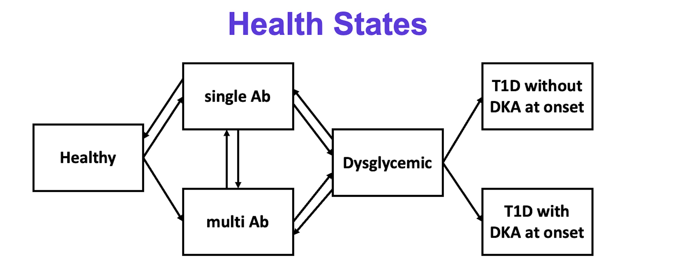
Figure 1: Representation of States in the Microsimulation. Every simulant starts in a healthy state and eventually transitions to various possible intermediate disease states (single auto-antibody(Ab1), multi auto-antibody(mAb1) and dysglycemic) up until the type 1 diabetes state with or without a diabetic ketoacidosis (DKA) event at onset.
Modeling Children
With microsimulations being agend-based simulations, creating and managing a population of simulants (i.e digital children) and their attributes is a critical task. Each digital child have its own individual clinical/demographic/genetic features such as age, genetic risk score, and family history for T1D. Importantly, these attributes are based on real-world data distributions. The idea is that based on individual transition probabilities, we simulate individuals through the model one at a time and we keep track of their individual trajectories so that at the end we aggregate results for the entire population. The core representation of simulants and their state information is a simple pandas dataframe. Under this representation rows represent children while columns correspond to state and/or any other attributes like the ones mentioned above. These columns represent one of several resources that other components can act up on. Each of the actions we need to take regarding the population of simulants corresponds to a manipulation of this pandas dataframe. For example, the addition of new simulants is the creation of new rows, the creation of new state attributes is the creation of columns, and the reading and updating of state attributes is reading and updating the dataframe itself. So now that we modelled both T1D and a population of children, how do we ensure that transition probabilities between states are reflective of what is observed in the real-world?
Transition probabilities
This is where we integrate machine learning into our microsimulation system. The main idea involves fitting survival regression models (LogNormal AFT) to real-world observational data. These are a class of models used in survival analysis, a collection of statistical methods that deals with the prediction of time until an event of interest take place. These are particularly useful in scenarios where you are not only interested in whether an event will happen, but also in how long it will take for that same event to happen. By fitting a LogNormal AFT model to observational data, we learn the relationship between the patient’s features and their likelihood of transitioning from one disease state to another. Once that is done, we integrate these models into our microsimulation system and feed them with the population of digital children, enabling us to compute individual transition probabilities for each child. Practically, we generate a predictive survival function for each individual which provides their probability of ‘surviving’ (or remaining in the same state) beyond a specified time t.
With the implementation of the disease modeling, the modeling of a population of children, and the computation of individual transition probabilities, we establish what is typically referred to as a baseline simulation. This baseline simulation can be used as benchmark against which interventions can be compared to and “what if” scenarios tested in a very rapid and cost-effective manner. By altering parameters of interest or introducing new variables, the impact of these changes can be evaluated relatively to the baseline.
Visualising the Simulations
The full implementation of the baseline simulation presents an excellent opportunity to move the system beyond the command-line and come up with ways of visualising the microsimulation system. This, in my opinion, greatly helps with the story telling and communication of microsimulation process in a more intuitive and engaging manner. The video below presents an animated plot, which grabs data from our microsimulation over a span of 15 years. Each point in the animated plot represents a single digital child and the transitions observed between health states result from the output of the survival regression models discussed above.
Up Next -> Model Validation
With the baseline model implemented we might be tempted to start testing multiple ‘what if’ scenarios which is perhaps the most powerfull feature of microsimulations. But before we do, can we really trust our model? Does it accurately reflect the real-world system it is trying to represent? In the next blog post, I will explore how to assess the validity of the model and its input data, and whether its predictions align well with real-world outcomes. Ultimately, we need to determine if our model is a true and reliable representation of the system we trying to simulate. Stay tuned.